Algorithms are a central object in Computer Science. They describe how to transform input data to output data, typically to solve a certain problem of interest (e.g., sorting a list of numbers in ascending order). While some algorithms are designed to terminate (e.g., sorting), some are designed to never terminate. Their input and output are streams of data (e.g., a database with add and query operations).
We will not go into details about how these algorithms are described as mathematical objects, but refer the interested reader to a quick overview of the most widely used model, the Turing machine, at Wikipedia.
Once we have an algorithm, and maybe even its implementation, e.g., in Python, we are interested in how good it is. This is typically measured in terms of the computation time and memory space it requires to run. But other complexity/performance measures are useful in other contexts. For example, for distributed algorithms that run on several machines, the number and size of exchanged messages is relevant.
Since we often want to compare algorithms (and not a particular input on a specific machine with a fixed implementation), one often abstracts away details in these complexity measures. Mostly this is done by looking only at the behavior of the complexity measure for large input sizes, i.e., at its asymptotic behavior for input sizes growing to infinity.
This allows us to focus on the essentials and make algorithms comparable in the first place. Keep in mind, though, that this abstract view has limitations. For example, an algorithm that may be asymptotically better, may show worse performance on small input sizes.
Complexity as a function
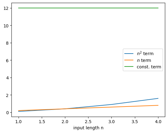
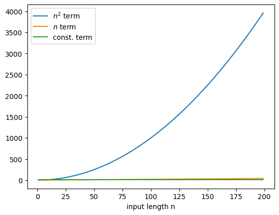
Assume that we have determined un upper bound \(f\) on the time \(T\), say in seconds, it takes for an algorithm to sort a list of length \(n\). Assume it is of this form:
It is by far the quadratic term that now determines the bound \(f\). We can thus simply say, the asymptotic time complexity is bounded by a quadratic term in \(n\).
This is formalized in the following.
Big-O notation (\(O\))
Definition
For a function \(f(n)\), we say \(f(n)\) is (in) \(O(g(n))\) if there exist constants \(c > 0\) and \(n_0 \geq 0\) such that:
\[
f(n) \leq c \cdot g(n) \quad \text{for all } n \geq n_0
\]
One also writes \(f(n) = O(g(n))\), but be careful that this equality sign is not symmetric like the usual equality sign. Another way of thinking about this is as \(O(g(b))\) as a class of functions, and instead of \(f \in O(g)\), we write \(f(n) = O(g)\).
Intuition
Big-O gives an upper bound on the growth of a function for large \(n\).
Example
Show that \(f(n) = 0.1n^2 + 0.2n + 12\) is in \(O(n^2)\).
Proof
We want to find constants \(c\) and \(n_0\) such that:
\[
0.1n^2 + 0.2n + 12 \leq c \cdot n^2 \quad \text{for all } n \geq n_0
\]
Divide both sides by \(n^2 > 0\). Then the above is equivalent to:
\[
0.1 + \tfrac{0.2}{n} + \frac{12}{n^2} \leq c
\]
Thus if we choose \(c = 1.3\) and \(n_0 = 12\), the first inequality in the proof is fulfilled.
Therefore, \(f(n) = O(n^2)\).
Big-Omega notation (\(\Omega\))
Definition
For a function \(f(n)\), we say \(f(n)\) is \(\Omega(g(n))\) if there exist constants \(c > 0\) and \(n_0 \geq 0\) such that:
\[
f(n) \geq c \cdot g(n) \quad \text{for all } n \geq n_0
\]
Intuition
Big-Omega gives a lower bound on growth. We typically want to use it on lower bounds of complexity bounds. For example, we would typically not apply it to the upper time bound \(f(n) = 0.1n^2 + 0.2n + 12\) from before, but on a lower time bound.
Example Assume we showed that our algorithm always needs at least \(f(n) = 5n + 3\) time (in seconds) to compute an answer. Show that \(f(n) = 5n + 3\) is \(\Omega(n)\).
Proof
We want constants \(c, n_0\) such that:
\[
5n + 3 \geq c \cdot n \quad \text{for all } n \geq n_0
\]
Divide by \(n > 0\):
\[
5 + \tfrac{3}{n} \geq c
\]
For all \(n \geq 1\), we have \(5 + \tfrac{3}{n} \geq 5\). So we can choose \(c = 5\) and \(n_0 = 1\) to fulfill the definition of \(\Omega\). Therefore, \(5n+3 = \Omega(n)\).
Big-Theta notation (\(\Theta\))
Definition
For a function \(f(n)\), we say \(f(n)\) is \(\Theta(g(n))\) if there exist constants \(c_1, c_2 > 0\) and \(n_0 \geq 0\) such that:
\[
c_1 \cdot g(n) \leq f(n) \leq c_2 \cdot g(n) \quad \text{for all } n \geq n_0
\]
Intuition
Big-Theta gives a tight asymptotic bound: “f grows at the same rate as g, up to constant factors.”
Example
Show that \(f(n) = 5n + 3\) is \(\Theta(n)\).
Proof
From the Big-Omega proof we had:
\[
5n + 3 \geq 5n \quad \text{for all } n \geq 1
\]
Using a similar proof we can show Big-O:
\[
5n + 3 \leq 8n \quad \text{for all } n \geq 1
\]
With \(c_1 = 5\), \(c_2 = 8\), and \(n_0 = 1\), both bounds hold:
\[
5n \leq 5n+3 \leq 8n
\]
Therefore, \(5n+3 = \Theta(n)\).
Complexity of an algorithm
Asymptotic notations can be useful to compare the performance of algorithms. We will do this at the example of a basic problem from computational biology.
Problem: GC in prefix.
Assume we are given a genetic sequence \(s = GTTCAT \dots\) and we would like to compute the number of G or C bases up to some position \(i \geq 0\). The result may be used to determine the GC-content in a subseqeunce from \(i\) to \(j \geq i\).
Let us assume that the input sequence length is \(n\). Assuming that basic operations (+, append, ==, etc.) require constant time, we observe that if is executed \(1 + 2 + 3 + \dots + n = O(n^2)\) times.
By contrast the following algorithm
def gc_prefix_good(seq): res: list[int] = [] count: int=0for ch in seq:if ch =="G"or ch =="C": count +=1 res.append(count)return res
executed the inner if only \(n = O(n)\) times.
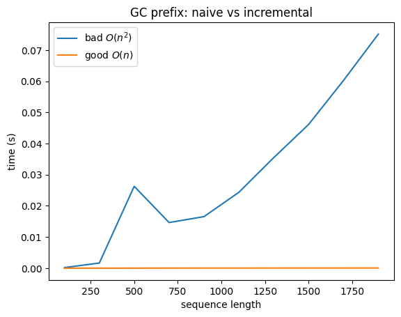
We can thus say that the first algorithm has time complexity \(O(n^2)\) and the second one \(O(n)\). So let us benchmark the two algorithms if we indeed say what we expect from asymptotic considerations.
Can we even do better? In fact under the assumption that we have to look at least once at each of the sequence positions (assuming that we do not have any further information on the sequence), one can show that \(n\) is in deed optimal: we can thus say we found an algorithm with optimal time complexity. Mind that this does not outrule the fact that someone cannot beat our algorithm via coding it in Rust, using parallel computation, etc. All we say is that asymptotically this does not change anymore the runtime besides constant factors.