Ordinary Differential Equations

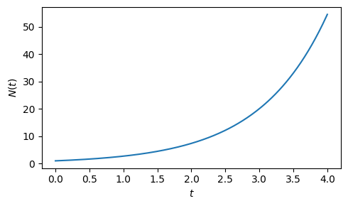
In terms of mathematics, differential equations are a relatively young but very powerful tool that began with Isaac Newton and Gottfried Leibniz. They are the method of choice for modeling physics today. We review some basics in this chapter.

Why differential equations?

Many processes in nature evolve continuously over time. For a state \(x \in \mathbb{R}^n\), with some dimensioninality \(n > 0\), and denoting by \(x(t)\) the state at time \(t > 0\), this corresponds to a continuous evolution of the function \(t \mapsto x(t)\). When we want to understand how something changes, whether it is the concentration of a protein in a cell, the number of individuals in a population, or the velocity of a falling object, we often find that the rate of change depends on the current state of the system. This leads us naturally to differential equations.

An ordinary differential equation (ODE) is simply an equation that relates a function to its derivatives. The word “ordinary” distinguishes these from partial differential equations, which involve derivatives with respect to multiple variables. In this primer, we focus exclusively on ODEs, which are sufficient for modeling systems that evolve in time alone.

First-order ODEs

The simplest and most fundamental type of ODE is the first-order equation, which involves only the first derivative. For a one-dimensional state \(x \in \mathbb{R}\), we write this as:

\[\frac{dx}{dt} = f(x)\]

The derivative \(dx/dt\) represents the instantaneous rate of change of \(x\) with respect to time. It is set equal to a function \(f\) of the current state.

Example: Exponential growth

Consider a simple example from biology that falls into this category: a bacterial population growing in unlimited resources. If we let \(N(t)\) represent the number of bacteria at time \(t\), we might model the growth rate as proportional to the current population size. This gives us

\[\frac{dN}{dt} = r N \,,\]

where \(r\) is the growth rate constant. This is one of the most famous ODEs in biology, and its solution is exponential growth:

\[N(t) = N_0 e^{rt}\,,\]

where \(N_0\) is the initial population size. You can verify that this is indeed a solution by substituting into the ODE. Doing so, we get:

\[\frac{d}{dt} \left( N_0 e^{rt} \right) = N_0 \cdot \frac{d}{dt} \left( e^{rt} \right) = r N_0 e^{rt} = r N\]

Plotting the solution results in the expected exponential growth curve over time.

Code

import numpy as np
import matplotlib.pyplot as plt

t = np.linspace(0, 4, 300)
r = 1.0
N0 = 1.0

plt.figure(figsize=(5, 3))
plt.plot(t, N0 * np.exp(r * t), label=rf'$r={r}$')
plt.xlabel(r'$t$')
plt.ylabel(r'$N(t)$')
plt.tight_layout()

Exponential growth cannot persist indefinitely: a bacterial culture in a flask will eventually exhaust its nutrients and slow down growth. We can also express this with a slightly more complex ODE as discussed in the following example.

Example: Logistic growth

Exponential growth cannot persist indefinitely: a bacterial culture in a flask will eventually exhaust its nutrients and stall. So let us write down a one-dimensional ODE that grows exponentially for small populations but saturates at some maximum, the carrying capacity \(K\).

The key observation is that the growth rate must vanish as \(N \to K\) and remain positive for \(N < K\). The simplest factor that does this is \((1 - N/K)\), which equals \(1\) at \(N = 0\) and \(0\) at \(N = K\). Multiplying the exponential rate \(rN\) by this factor gives

\[\frac{dN}{dt} = r N \!\left(1 - \frac{N}{K}\right), \qquad N(0) = N_0 > 0.\]

Expanding the right-hand side as \(rN - (r/K)N^2\) makes the nonlinearity explicit: this is no longer a linear ODE. The solution of this ODE is a bit more involved, but known.

Solution. Divide both sides by \(N(1-N/K)\):

\[\frac{1}{N\!\left(1 - N/K\right)}\frac{dN}{dt} = r.\]

Writing \(1 - N/K = (K-N)/K\), partial fractions give

\[\frac{K}{N(K-N)} = \frac{1}{N} + \frac{1}{K-N},\]

verified immediately by adding the two fractions. The equation becomes

\[\frac{1}{N}\frac{dN}{dt} + \frac{1}{K-N}\frac{dN}{dt} = r.\]

By the chain rule and integration tables (\(\frac{d}{dN}\ln N = \frac{1}{N}\)), each term on the left is the time derivative of a known function:

\[\frac{1}{N}\frac{dN}{dt} = \frac{d}{dt}\ln N, \qquad \frac{1}{K-N}\frac{dN}{dt} = \frac{d}{dt}\bigl[-\ln(K-N)\bigr].\]

So the equation reads \(\dfrac{d}{dt}\!\left[\ln N - \ln(K-N)\right] = r\). Integrating both sides from \(0\) to \(t\):

\[\ln\frac{N}{K-N} - \ln\frac{N_0}{K-N_0} = rt.\]

Exponentiating both sides:

\[\frac{N}{K-N} = \frac{N_0}{K-N_0}\,e^{rt}.\]

\[\begin{align} N &= \frac{N_0}{K-N_0}\,e^{rt}(K - N) \\[4pt] N\bigl(K - N_0 + N_0\,e^{rt}\bigr) &= N_0 K\,e^{rt} \\[4pt] N &= \frac{N_0 K\,e^{rt}}{K - N_0 + N_0\,e^{rt}}. \end{align}\]

Dividing numerator and denominator by \(N_0\,e^{rt}\) gives the exact solution:

\[\boxed{N(t) \;=\; \frac{K}{1 + \!\left(\dfrac{K}{N_0} - 1\right)e^{-rt}}.}\]

This S-shaped (sigmoidal) curve is one of the most important shapes in quantitative biology. For \(N_0 \ll K\) it is indistinguishable from exponential growth; as \(N \to K\), growth decelerates and \(N\) asymptotes to \(K\) regardless of \(N_0\). The inflection point, where growth is fastest, occurs at \(N = K/2\), independent of \(r\) and \(N_0\).

We will return to this example in the qualitative analysis and numerical sections below.

Plotting results in bounded growth over time. The level of maximum growth rate at \(K/2\) and the carrying capacity at \(K\) are marked with dotted lines.

Code

t = np.linspace(0, 10, 300)
K, r, N0 = 1.0, 1.0, 0.1
plt.figure(figsize=(5, 3))
N = K / (1 + (K / N0 - 1) * np.exp(-r * t))
plt.plot(t, N)
plt.xlabel('$t$')
plt.ylabel('$N(t)$')

plt.axhline(K, color='k', lw=0.8, ls='--', label='$K$')
plt.axhline(K/2, color='k', lw=0.8, ls='--', label='$K/2$')

plt.tight_layout()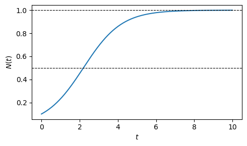

Solving ODEs

The two examples above illustrate two distinct strategies for finding exact solutions.

Ansatz. For the exponential growth equation \(\dot{N} = rN\), we guessed the form \(N(t) = N_0 e^{rt}\) and verified it by substitution. This works whenever the structure of the equation suggests a natural candidate: exponentials for linear equations, powers, trigonometric functions. It is the fastest route when it applies.

Rewriting as a time derivative. The logistic equation required a different strategy. After dividing both sides by \(N(1-N/K)\) and applying partial fractions, the chain rule turned each term on the left into the time derivative of a known function:

\[g(N)\,\dot N = \frac{d}{dt}G(N(t)) \quad \text{whenever } G' = g,\]

which could then be integrated directly using tables. The result was an algebraic equation for \(N(t)\).

Linear first-order ODEs. A particularly important special case is

\[\frac{dx}{dt} = ax + b, \qquad x(0) = x_0,\]

which describes, for example, protein production at constant rate \(b > 0\) with linear degradation for an \(a < 0\). The structure is simple enough to yield an exact closed-form solution. The unique equilibrium satisfies \(\dot x = 0\), giving \(x^* = -b/a\). Shifting to \(y = x - x^*\) removes the constant:

\[\frac{dy}{dt} = \frac{dx}{dt} = a(y + x^*) + b = ay.\]

This is exactly the exponential-growth equation, with solution \(y(t) = y_0\,e^{at}\). Converting back to \(x\):

\[\boxed{x(t) = x^* + (x_0 - x^*)\,e^{at}.}\]

For \(a < 0\) the solution relaxes exponentially toward \(x^*\) with time constant \(\tau = 1/|a|\). For \(a > 0\) it diverges from it.

When closed-form solutions fail. The logistic equation was special: its nonlinearity produced recognizable time derivatives after partial fractions. Most nonlinear ODEs lack this property and cannot be solved in closed form. This is not a limitation of technique but a fundamental feature of nonlinear dynamics. When exact solutions are unavailable, we turn to qualitative analysis and numerical methods.

Qualitative analysis: understanding without solving

Even when we cannot solve an ODE explicitly, we can often understand its solutions’ behavior through qualitative analysis. For first-order equations \(dx/dt = f(x)\), we can sketch the phase line — a diagram showing where \(f(x)\) is positive (so \(x\) increases), negative (so \(x\) decreases), or zero (so \(x\) remains constant).

Points where \(f(x) = 0\) are called equilibrium points. Their stability is determined by the sign of \(f'(x^*)\): if \(f'(x^*) < 0\), the equilibrium is stable; if \(f'(x^*) > 0\), it is unstable.

Example: Gene expression

Consider \(\dot x = \beta - \gamma x\), representing protein production at rate \(\beta\) and linear degradation at rate \(\gamma x\). The right-hand side \(f(x) = \beta - \gamma x\) is a line with negative slope \(-\gamma\), crossing zero at the unique equilibrium \(x^* = \beta/\gamma\). Since \(f'(x^*) = -\gamma < 0\), the equilibrium is stable: any initial protein concentration relaxes exponentially toward \(x^*\). Note that here we can also directly read off the solution from the linear ODE section: \(x(t) = x^* + (x_0 - x^*)\,e^{-\gamma t}\).

Code

beta, gamma = 1.0, 0.5
x_star = beta / gamma
x = np.linspace(0, 2 * x_star + 0.5, 300)
f = beta - gamma * x

plt.figure(figsize=(5, 2.5))
plt.axhline(0, color='k', lw=0.8)
plt.fill_between(x, f, where=(f > 0), color='C0', alpha=0.15, label=r'$\dot x > 0$')
plt.fill_between(x, f, where=(f < 0), color='C3', alpha=0.15, label=r'$\dot x < 0$')
plt.plot(x, f, 'k')
plt.plot(x_star, 0, 'o', mfc='k', mec='k', ms=8)   # stable
plt.xlabel('$x$')
plt.ylabel('$f(x)$')
plt.legend()
plt.tight_layout()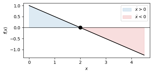

Example: Phase line for logistic growth

Recall the logistic growth ODE with

\[f(N) = rN(1-N/K).\]

Here, the zeros are \(N=0\) and \(N=K\).

Between them \(f > 0\) so the population grows; above \(K\), \(f < 0\) so it shrinks. The derivative \(f'(N) = r(1 - 2N/K)\) gives \(f'(0) = r > 0\) (unstable) and \(f'(K) = -r < 0\) (stable). Every trajectory with \(N_0 > 0\) therefore converges to \(K\), confirming what we already read off the explicit solution.

Code

K, r = 1.0, 1.0
N = np.linspace(0, 1.5, 300)
f = r * N * (1 - N / K)

plt.figure(figsize=(5, 2.5))
plt.axhline(0, color='k', lw=0.8)
plt.fill_between(N, f, where=(f > 0), color='C0', alpha=0.15, label=r'$\dot N > 0$')
plt.fill_between(N, f, where=(f < 0), color='C3', alpha=0.15, label=r'$\dot N < 0$')
plt.plot(N, f, 'k')
plt.plot(0, 0, 'o', mfc='white', mec='k', ms=8)   # unstable
plt.plot(K, 0, 'o', mfc='k',     mec='k', ms=8)   # stable
plt.xlabel('$N$')
plt.ylabel('$f(N)$')
plt.legend()
plt.tight_layout()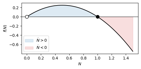

Systems of ODEs: coupled dynamics

Real biological and physical systems rarely involve just one variable changing over time. More often, we have multiple interacting components, leading to systems of coupled ODEs. For two variables, this takes the form:

\[\frac{dx}{dt} = f(x, y)\] \[\frac{dy}{dt} = g(x, y)\]

Such systems can exhibit far richer behavior than single equations. Equilibrium points are now points in the \((x, y)\) plane where both \(dx/dt = 0\) and \(dy/dt = 0\). The stability of these equilibria is determined by linearization: we approximate the nonlinear system near the equilibrium using its linear part, then analyze the eigenvalues of the resulting Jacobian matrix.

The classic predator-prey model illustrates this beautifully. If \(x\) represents prey and \(y\) represents predators, we might write:

\[\frac{dx}{dt} = ax - bxy\] \[\frac{dy}{dt} = -cy + dxy\]

The prey grow exponentially in the absence of predators but are consumed at a rate proportional to predator-prey encounters. The predators die off without prey but grow through consumption. This system has a non-trivial equilibrium at \((c/d, a/b)\) around which populations oscillate periodically—a phenomenon that cannot occur in single first-order ODEs but emerges naturally in two-dimensional systems.

Linear systems and matrix exponentials

Linear systems of ODEs deserve special attention because they are exactly solvable and provide the foundation for understanding nonlinear systems through linearization. A linear system has the form:

\[\frac{d\mathbf{x}}{dt} = A\mathbf{x}\]

where \(\mathbf{x}\) is a vector and \(A\) is a constant matrix. The solution is given by the matrix exponential

\[\mathbf{x}(t) = e^{At}\mathbf{x}_0 .\]

The behavior of this system is entirely determined by the eigenvalues of \(A\). If all eigenvalues have negative real parts, solutions decay to zero—the system is stable. If any eigenvalue has a positive real part, solutions grow without bound—the system is unstable. Complex eigenvalues lead to oscillatory behavior, with the real part determining whether the oscillations grow or decay.

This eigenvalue analysis extends to nonlinear systems through linearization. Near an equilibrium point, we approximate the nonlinear system by its linear part, and the eigenvalues of the Jacobian matrix determine local stability. This is why linear algebra is indispensable for understanding ODEs.

Higher-order ODEs and dimensionality

A second-order ODE involves the second derivative and is of the form

\[\frac{d^2x}{dt^2} = f(x, dx/dt, t).\]

Such equations arise naturally in mechanics, where Newton’s law \(F = ma\) gives acceleration \(a = \frac{dv}{dt} = \frac{d^2x}{dt^2}\) as a function of position \(x\) and velocity \(v\). For instance, a simple harmonic oscillator satisfies

\[F = -k x ,\]

where the force pushes proportionally to the displacement towards the center. For example, a mass on a spring shows such behavior.

This yields

\[ -k x = m \frac{d^2x}{dt^2} \]

and by setting \(\omega^2 = \frac{k}{m}\),

\[\frac{d^2x}{dt^2} = -\omega^2 x.\]

Any higher-order ODE can be converted into a system of first-order ODEs by introducing new variables for each derivative. The second-order equation above becomes a first-order system by setting \(v = dx/dt\):

\[\frac{dx}{dt} = v\] \[\frac{dv}{dt} = -\omega^2 x\]

This transformation is more than mathematical convenience—it reveals that second-order equations are fundamentally two-dimensional dynamical systems. The phase space for this oscillator is the \((x, v)\) plane, and solutions trace out circular or elliptical orbits representing periodic motion.

Code

from matplotlib.animation import FuncAnimation
from IPython.display import HTML

omega, n = 1.0, 200
t = np.linspace(0, 2 * np.pi, n)
x, v = np.cos(omega * t), -np.sin(omega * t)

fig, (ax1, ax2) = plt.subplots(1, 2, figsize=(8, 3))
ax1.plot(t, x, 'k', lw=0.5, alpha=0.3)
ax1.set_xlabel('$t$'); ax1.set_ylabel('$x(t)$')
dot1, = ax1.plot([], [], 'o', color='C0', ms=7)

ax2.plot(x, v, 'k', lw=0.5, alpha=0.3)
ax2.set_xlabel('$x$'); ax2.set_ylabel('$v$'); ax2.set_aspect('equal')
dot2, = ax2.plot([], [], 'o', color='C0', ms=7)
trail, = ax2.plot([], [], color='C0', lw=1.5, alpha=0.5)
fig.tight_layout()

def update(i):
    dot1.set_data([t[i]], [x[i]])
    dot2.set_data([x[i]], [v[i]])
    trail.set_data(x[max(0, i - 50):i + 1], v[max(0, i - 50):i + 1])
    return dot1, dot2, trail

ani = FuncAnimation(fig, update, frames=n, interval=30, blit=True)
plt.close()
HTML(ani.to_jshtml())

Numerical methods: computing solutions

When analytical solutions are unavailable, numerical methods approximate solutions at discrete time points. The simplest method is Euler’s method: starting from an initial condition \(x_0\) at \(t_0\), we approximate \(x(t_0 + h) \approx x_0 + h \cdot f(x_0)\) for small time step \(h\). This follows directly from the definition of the derivative.

While Euler’s method is intuitive, more sophisticated methods like Runge-Kutta achieve better accuracy by evaluating the derivative at multiple points within each time step. The fourth-order Runge-Kutta method (RK4) is particularly popular, balancing accuracy and computational cost. Most modern ODE solvers use adaptive methods that automatically adjust the step size to maintain accuracy while minimizing computation.

Numerical solutions are essential for real applications, but they come with caveats. Stability of the numerical method is distinct from stability of the differential equation itself. Stiff equations—those with widely separated time scales—pose particular challenges, requiring specialized implicit methods that remain stable even with large time steps.

Applications in Biological Systems

ODEs are the primary mathematical tool for modeling dynamics in molecular and cell biology. The central dogma of molecular biology—DNA makes RNA makes protein—translates naturally into coupled differential equations. If we let \(m(t)\) represent mRNA concentration and \(p(t)\) represent protein concentration, we might write:

\[\frac{dm}{dt} = \beta_m - \gamma_m m\] \[\frac{dp}{dt} = \beta_p m - \gamma_p p\]

Here, \(\beta_m\) is the transcription rate, \(\gamma_m\) is the mRNA degradation rate, \(\beta_p\) is the translation rate per mRNA molecule, and \(\gamma_p\) is the protein degradation rate. This simple model captures the time scales of gene expression and predicts steady-state protein levels.

More complex regulatory networks require systems of many coupled ODEs. The repressilator, three genes repressing each other in a cycle that we will later analyze in this course, demonstrates how simple regulatory motifs can generate oscillations. Models of cell cycle control, metabolic networks, and signal transduction pathways all employ ODEs to bridge molecular mechanisms and cellular behavior.

Beyond ODEs: What comes next

This primer focuses on deterministic ODEs, where the same initial condition always produces the same trajectory. Real biological systems involve randomness—molecules diffuse, reactions occur probabilistically, and populations fluctuate. Stochastic differential equations and the chemical master equation extend ODEs to capture this randomness.

ODEs assume well-mixed systems where spatial position is irrelevant. When spatial structure matters—during development, tissue formation, or epidemic spread: we need partial differential equations or agent-based models. Nevertheless, ODEs often provide an essential first approximation, capturing the essential temporal dynamics before adding spatial complexity.

For systems with discrete events—such as cell division, viral infection, or threshold-crossing—hybrid models combining ODEs with discrete switches may be more appropriate. The choice of modeling framework depends on the biological question and the available data.

Key takeaways

Ordinary differential equations are the natural language for describing continuous change. They allow us to express mechanistic understanding, how rates of change depends on current state, and derive predictions about long-term behavior. While only special ODEs have closed-form solutions, qualitative analysis and numerical methods provide powerful tools for understanding any system.

For students of computational bioengineering, facility with ODEs is essential. They appear throughout systems biology, from gene regulation to population dynamics. The ability to formulate problems as ODEs, analyze their behavior, simulate them numerically, and connect them to data is fundamental to modern quantitative biology.