where the arguments are position \(\mathbf{r}\) and time \(t\). The quantity \(|\Psi(\mathbf{r},t)|^2\) is the probability density of finding the electron at position \(\mathbf{r}\) at time \(t\).
Schrödinger equation
Denoting by \(\nabla^2 = \frac{\partial^2}{\partial x^2}+\frac{\partial^2}{\partial y^2}+\frac{\partial^2}{\partial z^2}\) the Laplacian, the dynamics of the wavefunction are governed by the Schrödinger equation. The equation has derivatives in space and time and thus falls into the class of partial differential equations (PDEs). It reads:
where \(\hat{H}\) is the Hamiltonian operator, \(\hbar\) the reduced Planck constant, \(m_e\) the electron mass, and \(V\) the potential energy. The first term of \(\hat{H}\) is the kinetic energy operator. The potential \(V\) encodes all electrostatic interactions.
Example: double-slit
One of the most famous experiments in quantum physics is the double-slit experiment: a particle moves toward a hard wall with two narrow gaps and diffracts into an interference pattern typical for a wave.
It turns out that even for this simple setting, solving the PDE is out of reach. We thus turn to a numeric solution, also called a simulation.
However, the simulation would require us to store a state for each of the infinite times and positions in space which is clearly infeasible.
A classical abstraction is the following:
Abstraction: time and grid discretisation.
We replace each continuous axis by sample points: time in steps of some \(dt > 0\) and space in steps of some \(dx > 0\). For each time and space point we thus need to store a single complex number. The discretization in space transforms the PDE into a finite ODE system. The discretization in time finally allows us to numerically solve the system, e.g., by methods like Euler integration as we have discussed them in the Preliminaries.
The simulation below runs the full time-dependent equation in 2d to show the double-slit experiment with the particle modeled as a Gaussian wave packet (in atomic units, \(\hbar=m_e=1\)).
The simulator in src/schrodinger2d.py uses an interesting method introduced in (Visscher; Computers in Physics, 1991) and known as the Visscher leapfrog. Splitting \(\Psi = \Psi_R + i\Psi_I\) and staggering the two parts by \(dt/2\) gives a conditionally stable explicit update:
where \(H = -\tfrac{1}{2}\nabla^2\) and \(\nabla^2\) is the standard 5-point finite-difference Laplacian. The hard wall is enforced by setting \(\Psi=0\) on barrier grid points after every half-step. Stability requires \(dt \leq dx^2/2\).
Code
import importlibimport src.schrodinger2dimportlib.reload(src.schrodinger2d)from src.schrodinger2d import simulatefrom matplotlib import animationfrom IPython.display import HTMLimport numpy as npimport matplotlib.pyplot as plt# --- parameters: change these to explore ---nx, ny =128, 128# grid pointsdx =0.5# grid spacing in a0x0, y0 =None, None# electron start (None = centre / lower quarter)kx, ky =0.0, 3.0# initial momentum in atomic unitssigma =3.0# wave-packet width in a0n_steps =500n_frames =80# Barrier geometry: barrier(X, Y) -> bool array; True = hard wall (ψ = 0).# X, Y are meshgrids of shape (nx, ny).# Edit freely to draw any geometry.Lx, Ly = nx * dx, ny * dxcx = Lx /2wall_y =0.55* Lyslit_width =1.2# full width of each slit in a0slit_separation =3.0# centre-to-centre distance between slits in a0def barrier(X, Y):return ( (Y >= wall_y) & (Y < wall_y + dx)&~( (np.abs(X - (cx - slit_separation /2)) < slit_width /2)| (np.abs(X - (cx + slit_separation /2)) < slit_width /2) ) )# -------------------------------------------frames, x, y, mask = simulate( nx=nx, ny=ny, dx=dx, x0=x0, y0=y0, kx=kx, ky=ky, sigma=sigma, barrier=barrier, n_steps=n_steps, n_frames=n_frames,)vmax =max(f.max() for f in frames) *0.4# Dark-blue wall overlaywall_rgba = np.zeros((*mask.T.shape, 4))wall_rgba[mask.T] = [0.08, 0.18, 0.40, 1.0]fig, ax = plt.subplots(figsize=(5, 5))def update(frame): ax.clear() ax.set_facecolor("white") ax.imshow( frames[frame].T, origin="lower", extent=(x[0], x[-1], y[0], y[-1]), cmap="hot_r", vmin=0, vmax=vmax, ) ax.imshow( wall_rgba, origin="lower", extent=(x[0], x[-1], y[0], y[-1]), ) ax.set_xlabel(r"$x\,/\,a_0$") ax.set_ylabel(r"$y\,/\,a_0$") ax.set_title(r"$|\Psi|^2$")anim = animation.FuncAnimation(fig, update, frames=len(frames), interval=60)html = anim.to_jshtml()plt.close(fig)HTML(html)
Stationary states
One observes that the potential, i.e., the wall, did not move over time. While in biology potentials may change over time, they may change slow enough to be considered stationary.
For these stationary potentials, the Schrödinger equation can be simplified and admits separable (stationary) solutions. Since \(\hat{H}\) does not depend on \(t\), we can look for solutions of the form \(\Psi(\mathbf{r},t)=\psi(\mathbf{r})f(t)\). Substituting into the Schrödinger equation yields
which is essential for describing dynamical phenomena such as wave-packet propagation and interference.
Abstraction: stationary states. The full Schrödinger equation governs arbitrary time-varying states: superpositions, pulses, transitions. Restricting to stationary states (energy eigenstates) discards all dynamics: the system must already be in a definite energy eigenstate and stay there forever. This abstraction is valid for ground-state electronic structure (atoms and stable molecules at rest) but not for processes such as light absorption, during chemical reactions, or electron transfer, which require the full time-dependent equation. For our purposes, we can often make this abstraction since transient states vanish quickly.
These solutions are called stationary states: the full wavefunction \(\Psi(\mathbf{r},t)=\psi(\mathbf{r})e^{-iEt/\hbar}\) oscillates in time at a single frequency \(\omega = E/\hbar\), but the phase factor cancels in the probability density,
which is time-independent. The electron distribution is therefore frozen: the wavefunction oscillates uniformly everywhere at frequency \(\omega\), but nothing observable changes in time. This is the quantum analogue of a standing wave, where the amplitude pattern \(\psi(\mathbf{r})\) is fixed and only the phase rotates. Any solution of the full Schrödinger equation can be written as a superposition of such stationary states.
Indeed, biology seldomly requires knowing the quantum-transients like in the double-slit experiments, but is more about slowly (in terms of electron movement) changing molecules where electrons are quickly in steady-states.
Hydrogen atom
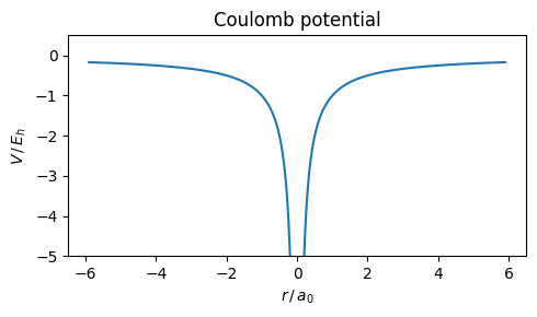
Biology is all about atoms interacting in fascinating ways. The simplest atom is a proton with an electron: a single hydrogen H. For one electron bound to a proton at the origin, the potential is the Coulomb attraction
\[V(r) = -\frac{e^2}{4\pi\epsilon_0\, r},\]
where \(r = |\mathbf{r}|\in[0,\infty)\) is the scalar distance, or radius, from the proton.
Plotting this over space \(r\) (in units of the Bohr radius\(a_0 = 4\pi\epsilon_0\hbar^2/(m_e e^2) \approx 53\,\text{pm}\), and thus energy in units of the Hartree\(E_h = e^2/(4\pi\epsilon_0 a_0) = m_e e^4/\bigl((4\pi\epsilon_0)^2\hbar^2\bigr) \approx 27.2\,\text{eV}\)) shows the characteristic \(1/r\) shape at the nucleus and the approach to zero for \(r \to \infty\).
Code
import numpy as npimport matplotlib.pyplot as pltr = np.linspace(-6, -0.1, 500) + np.linspace(0.1, 6, 500) # in units of a0plt.figure(figsize=(5, 3))plt.plot(r, -1/ np.abs(r))plt.ylim(-5, 0.5)plt.xlabel(r"$r\,/\,a_0$")plt.ylabel(r"$V\,/\,E_h$")plt.title("Coulomb potential")plt.tight_layout()plt.show()
The TISE for hydrogen is solved in spherical coordinates by writing the wavefunction as a product
which separates the equation into independent ODEs for \(R\), \(\Theta\), and \(\Phi\). The integers \(l\geq 0\) and \(|m|\leq l\) arise from two conditions on the angular factors:
Single-valuedness: the ODE for \(\Phi\) is \(\Phi''=-m^2\Phi\), solved by \(\Phi(\phi)=e^{im\phi}\). Since \(\phi\) and \(\phi+2\pi\) label the same point in space, \(\Phi\) must satisfy \(\Phi(\phi+2\pi)=\Phi(\phi)\), i.e., \(e^{2\pi im}=1\), which forces \(m\in\mathbb{Z}\).
Finiteness at the poles: the ODE for \(\Theta\) is the associated Legendre equation. Its solutions diverge at \(\theta=0\) and \(\theta=\pi\) unless \(l\) is a non-negative integer with \(l\geq|m|\), in which case they reduce to the associated Legendre polynomials \(P_l^m(\cos\theta)\). The combined angular solution \(Y_l^m(\theta,\phi) = P_l^m(\cos\theta)\,e^{im\phi}\) is called a spherical harmonic.
The radial part yields a third integer \(n\geq l+1\): for generic values of \(n\) the radial solution grows exponentially as \(r\to\infty\), making \(\int_0^\infty |R|^2 r^2\,\mathrm{d}r\) diverge and the state unphysical. Only when \(n\) is a positive integer with \(n\geq l+1\) does the solution decay exponentially, so that \(R_{nl}\) is square-integrable.
Together, the three quantum numbers \((n,l,m)\) fully label each bound state. Remarkably, the energy depends only on \(n\):
\[E_n = -\frac{E_1}{n^2}, \qquad n = 1, 2, 3, \ldots\]
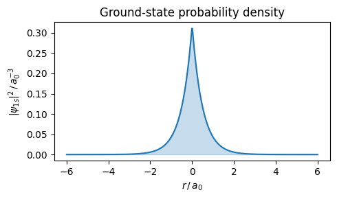
The ground state is the eigenfunction with the lowest energy (\(n=1\), \(l=m=0\)). At \(l=m=0\) the spherical harmonic reduces to a constant, \(Y_0^0(\theta,\phi)=1/\sqrt{4\pi}\), so \(\psi_{1s} = R_{10}(r)\cdot Y_0^0\) has no angular dependence — it is spherically symmetric. Substituting the radial solution \(R_{10}(r) = 2a_0^{-3/2}e^{-r/a_0}\) gives:
with \(a_0\) the Bohr radius. The probability density \(|\psi_{1s}|^2\) is spherically symmetric and decays exponentially. The following figure shows this probability density for the electron.
Code
r = np.linspace(-6, 6, 500) # in units of a0plt.figure(figsize=(5, 3))plt.plot(r, np.exp(-2* np.abs(r)) / np.pi)plt.fill_between(r, np.exp(-2* np.abs(r)) / np.pi, alpha=0.25, color='C0')plt.xlabel(r"$r\,/\,a_0$")plt.ylabel(r"$|\psi_{1s}|^2\,/\,a_0^{-3}$")plt.title("Ground-state probability density")plt.tight_layout()plt.show()
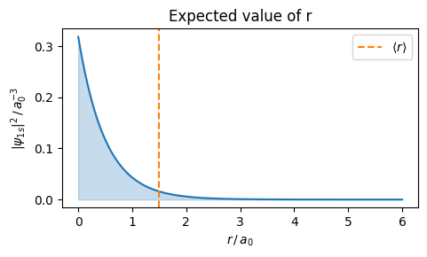
A natural question is where the electron is in expectation. To answer that one can compute expected value \(\langle r\rangle\) of \(r\) in state \(\psi_{1s}\).
As before, introduce spherical coordinates via the substitution \((x,y,z) = (r\sin\theta\cos\phi,\, r\sin\theta\sin\phi,\, r\cos\theta)\) with \(r\in[0,\infty)\), \(\theta\in[0,\pi]\), \(\phi\in[0,2\pi)\). The Jacobian of this substitution is
so by the change-of-variables theorem\(\int_{\mathbb{R}^3} f\,\mathrm{d}x\,\mathrm{d}y\,\mathrm{d}z = \int_0^\infty\int_0^\pi\int_0^{2\pi} f\, r^2\sin\theta\,\mathrm{d}\phi\,\mathrm{d}\theta\,\mathrm{d}r\). Since \(|\psi_{1s}|^2\) depends only on \(r\), the angular integrals factor and evaluate to \(\int_0^{2\pi}\mathrm{d}\phi\int_0^\pi\sin\theta\,\mathrm{d}\theta = 2\pi\cdot 2 = 4\pi\). The expected value therefore reduces to
where the last integral follows from \(\int_0^\infty r^3 e^{-\alpha r}\,\mathrm{d}r = 6/\alpha^4\).
The dotted line in the next figure shows the expected position of the electron.
Code
r = np.linspace(0, 6, 1000) # in units of a0dr = r[1] - r[0]psi2_1s = np.exp(-2* np.abs(r)) / np.pir_expect = np.sum(np.abs(r) * psi2_1s *4* np.pi * r**2) * drprint(f'<r> = {r_expect:.4f} a0')plt.figure(figsize=(5, 3))plt.title("Expected value of r")plt.plot(r, psi2_1s)plt.fill_between(r, psi2_1s, alpha=0.25, color='C0')plt.axvline(r_expect, color='C1', ls='--', label=r'$\langle r\rangle$')plt.xlabel(r'$r\,/\,a_0$')plt.ylabel(r'$|\psi_{1s}|^2\,/\,a_0^{-3}$')plt.legend()plt.tight_layout()plt.show()
<r> = 1.4966 a0
Chemical bonds
Biology requires more than unrelated single atoms. The complexity of life is based on complex molecules that are built from many atoms. For example, the amino acid Alanine (Ala) has 13 atoms.
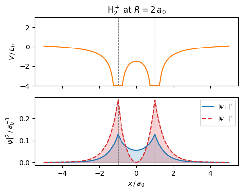
The simplest chemical bond is one with two protons that share an electron. This molecule is called \(\textrm{H}_2^+\). The electron, for the two protons A and B at distance \(R\), has potential
where \(r_A = |\mathbf{r}-\mathbf{r}_A|\) and \(r_B = |\mathbf{r}-\mathbf{r}_B|\) are the distances from the electron at position \(\mathbf{r}\) to each proton. So \(V(\mathbf{r})\) is the potential energy of the electron at \(\mathbf{r}\), with the two protons held fixed. The last term \(e^2/(4\pi\epsilon_0 R)\) is the (constant) proton–proton repulsion for fixed separation \(R\).
Abstraction: LCAO. The exact wavefunction for H\(_2^+\) lives in \(\mathbb{R}^3\) and satisfies a PDE with no closed-form solution in Cartesian coordinates. The LCAO approximation replaces it by a linear combination of known atomic orbitals:
This reduces an infinite-dimensional PDE to a \(2\times 2\) matrix problem (one coefficient per basis function) — exact only if the true wavefunction lies in the chosen subspace, which it does not.
Abstraction: linear, finite basis. Using only \(\psi_{1s}^A\) and \(\psi_{1s}^B\) as basis restricts the search to a two-dimensional subspace of the full function space. A richer basis (2s, 2p, \(\ldots\) orbitals on each centre) gives a larger matrix and a better energy, converging to the exact solution as the basis grows. The 1s-only LCAO is the coarsest useful choice.
The symmetric combination \(\psi_+\) (bonding orbital) concentrates electron density between the nuclei, lowering the total energy and forming a stable bond. The antisymmetric \(\psi_-\) (antibonding) has a nodal plane between the nuclei and higher energy.
The following figure shows this setting for the two protons being located at \(-a_0\) and \(a_0\), thus being within distance \(2 a_0\).
As \(R\) decreases from far-separated atoms toward the equilibrium bond length, three stages are visible:
Large \(R\): two separate density peaks, each electron cloud hugging its own nucleus — two independent H atoms.
Intermediate \(R\) (\(\approx 2\,a_0\)): the peaks merge and electron density builds up between the nuclei. This accumulation screens the proton-proton repulsion and lowers the total energy — the bond forms.
Small \(R\): the proton-proton repulsion \(1/R\) dominates and the potential rises steeply, preventing the nuclei from collapsing into each other.
The stable molecule sits at the \(R\) that minimises the total LCAO energy
i.e., the \(R^*\) satisfying \(\mathrm{d}E_+/\mathrm{d}R = 0\). As \(R\) decreases, the electron-nucleus attraction terms lower the energy while \(1/R\) raises it; the minimum is where these competing effects balance.
For a single electron the wavefunction \(\psi:\mathbb{R}^3\to\mathbb{C}\) lives in 3 dimensions. For \(N\) electrons it becomes
\[\Psi:\mathbb{R}^{3N}\to\mathbb{C},\]
since each electron \(i\) has its own position \(\mathbf{r}_i\in\mathbb{R}^3\) and all positions are coupled. The Hamiltonian acquires electron–electron repulsion terms:
where \(r_{i\alpha}\) is the distance from electron \(i\) to nucleus \(\alpha\) and \(r_{ij}=|\mathbf{r}_i-\mathbf{r}_j|\). The last sum couples all electron pairs — the equation no longer separates.
Solving the equation numerically. To represent \(\Psi\) numerically on a computer, one typically replaces each continuous space axis by \(k\) equally spaced sample points (e.g. \(x_1 < x_2 < \cdots < x_k\) covering the relevant range), storing the value of \(\Psi\) at each combination: a so-called grid or mesh.
Abstraction: grid discretisation. Replacing each continuous axis by \(k\) sample points turns the TISE, a PDE over \(\mathbb{R}^{3N}\), into a matrix eigenvalue problem of size \(k^{3N}\times k^{3N}\). The differential operators become finite differences and \(\Psi\) becomes a vector of \(k^{3N}\) complex numbers. This is exact in the limit \(k\to\infty\) but computationally intractable for any \(N>1\) at useful \(k\).
Each electron contributes 3 axes, so the full grid has \(k^{3N}\) points, with one complex number per point. For a carbon atom (with \(N=6\) electrons) and a course grid of \(k=100\) points per axis, one obtains \(100^{18} = 10^{36}\) numbers, which is beyond the possibility of any existing computer. Even for \(N=2\) electrons (e.g., two colliding H), one already needs a 6-dimensional grid.